MySQL, like any other technology, is constantly evolving and brings many new features. However, not everyone has the time to keep up with all the new features in this popular open-source database. Fortunately, this article provides a quick catch-up!

Before we dive into the features, let’s first look at how versioning works in MySQL. This will provide insights into some interesting facts. The first public version 8.0.11 of the latest major version of MySQL 8 was released on 19.4.2018. Since that, there have been over twenty individual releases. In the terminology of semantic versioning, these releases would be called “patch” releases. Unfortunately, MySQL does not adhere to semantic versioning, where only major releases introduce breaking changes. As a result, breaking changes can occur even in patch releases, such as the removal of TLSv1 and TLSv1.1 in 8.0.28 or changes in the MySQL protocol in 8.0.24. Hence, caution should be exercised when upgrading to the latest version. On the other hand, “patch” versions can bring many interesting features, which we will now explore.

Generated columns

We will start with a “left over” feature introduce in MySQL 5.7.7 – generated columns [1]. Generated columns provide a way to store automatically generated data in a table. The value of this data is computed by a predefined expression and cannot be manually changed, but it can be indexed. To create a generated column, we use the keyword “GENERATED always AS (expression)“. An example of this can be seen in the following code, where we are creating a table with a virtual column “full_name” that is combined from the “name” and “surname” columns (Listing 1).

CREATE TABLE users (
   id        INT AUTO_INCREMENT PRIMARY KEY,
   name      VARCHAR(60) NOT NULL,
   surname   VARCHAR(60) NOT NULL,
   full_name VARCHAR(120) 
   GENERATED ALWAYS AS (CONCAT(name, ' ', surname))
);

If we select the data from the table, the last column will contain the full name of the user (Listing 2). There are certain limitations to the expressions used in virtual columns. They cannot reference another generated column, auto-increment columns, use columns outside the table, or contain non-deterministic functions such as NOW().

SELECT * FROM users;
+----+------------+-----------+----------------+
| id | name       | surname   | full_name      |
+----+------------+-----------+----------------+
|  1 | Jane       | Doe       | Jane Doe       |
|  2 | Janie      | Stiles    | Janie Stiles   |
|  3 | Richard    | Miles     | Richard Miles  |
+----+------------+-----------+----------------+

There are two types of generated columns: virtual and stored. The value of a virtual column is resolved during a read operation, while the value of a stored column is evaluated during an insert or update operation and then stored on disk. The type of the column can be specified as the last value in the column definition, as either “VIRTUAL” or “STORED“. Examples of how to use both types can be seen in the Listing 3.

CREATE TABLE users_alter (
   id         INT AUTO_INCREMENT PRIMARY KEY,
   name       VARCHAR(60) NOT NULL,
   surname    VARCHAR(60) NOT NULL,
   full_name  VARCHAR(120) 
   GENERATED ALWAYS AS (CONCAT(name , ' ', surname )) VIRTUAL,
   hash varchar(32) 
   GENERATED ALWAYS AS (MD5(CONCAT(name , ' ', surname ))) STORED
);

SELECT * FROM users_alter;

+----+------------+-----------+----------------+------------+
| id | name       | surname   | full_name      | hash       |
+----+------------+-----------+----------------+------------+
|  1 | Jane       | Doe       | Jane Doe       | f001124... |
|  2 | Janie      | Stiles    | Janie Stiles   | 55bac62... |
|  3 | Richard    | Miles     | Richard Miles  | f32f3cd... |
+----+------------+-----------+----------------+------------+

As virtual columns are not stored on disk, their usage does not require any additional storage space. Absence of storing the results also means that INSERT and UPDATE queries come with no overhead. However, read operations may be slower as the results need to be evaluated during the read. Stored columns, on the other hand, have a performance penalty only during data-modifying queries.

There are many potential use cases for virtual columns, including simplifying and unifying queries, caching complicated conditions, indexing complex values, and extracting values from JSON data columns. They also serve as a foundation for other features that we will explore later.

JSON support

JSON support [2] has been available since the release of MySQL 5.7.9, with significant improvements made in MySQL 8. It is implemented in the form of a native column data type, providing automatic validation and an optimised binary storage format. While individual values within a JSON document cannot be directly indexed, functional indexes can be used to achieve this. JSONPath can be used to select values within a JSON document.

Inserting JSON data is as straightforward as inserting regular strings and does not require any special care. Values within a JSON document can be used in a field list by using the column path operator (->) and a JSONPath to the field. However, this can result in values being wrapped in quotes, which can be inconvenient. This can be remedied by using the column inline path operator (->>) since MySQL 8.0. Both operators can be used in other parts of a query, such as the WHERE condition (Listing 4).

SELECT id, browser->>'$.os' os
FROM activity
WHERE browser->>'$.name'='Firefox';

+----+---------+
| id | os      |
+----+---------+
|  2 | Windows |
+----+---------+

A partial update is implemented using a set of JSON_* functions. The most useful of these functions is probably JSON_SET(json_doc, path, val), which replaces existing values and adds new ones as necessary. In our example, we will attempt to rename Firefox back to its original name, Phoenix (Listing 5).

UPDATE activity
SET `browser` = JSON_SET(
   `browser`,
   '$.name',
   'Phoenix'
)
WHERE browser->>'$.name'='Firefox';

The JSON_SET function expects a column name as its first parameter, in which the JSON data is stored. The second parameter is the JSONPath, where in our case, “$.name” represents the property name. The last parameter represents the value itself, which in our case is the string ‘Phoenix’. Other useful functions include JSON_INSERT, JSON_REPLACE, and JSON_REMOVE.

IPC NEWSLETTER

All news about PHP and web development

Generated columns can be easily combined with JSON data types, as the column inline path operator (->>) can be used in column expressions. This allows us to extract some of the properties and make them available as regular fields (Listing 6).

CREATE TABLE activity (
   id           int auto_increment primary key,
   event_name   ENUM('page-view', 'user-login'),
   user_id      int,
   properties   json,
   browser      json,
   browser_name varchar(20)
   GENERATED ALWAYS AS (`browser` ->> '$.name')
);

JSON support provides the ability to mix document databases with relational databases, offering at least in theory the benefits of both. However, this can be complex and caution should be exercised. Possible use cases include error logging, application event logging, and piloting new ideas.

Instant DDL

DDL stands for Data Definition Language and is an umbrella term for all schema-changing commands. Instant DDL allows for schema changes in InnoDB without making the data in the schema unavailable. It has been partially supported since 8.0.12 and was extended in 8.0.29, making it the first big addition since the initial release of MySQL 8.0 (8.0.11). There is no need to do anything special to enable online DDL, but it is advisable to understand what is happening under the hood.

InnoDB supports three algorithms: COPY, INPLACE, and INSTANT. The difference between INSTANT and the other algorithms is that INSTANT only performs metadata changes and does not touch the data file of the table. The only downside is that INSTANT is only supported for limited DDL operations, namely: adding a column, dropping a column, renaming a column, modifying a column default value, and renaming a table.

Some operations are not supported, such as tables that use compressed row format, tables with a FULLTEXT index, temporary tables, and stored columns. Additionally, there are unsupported combinations. For example, a column drop is an instant operation, but an index drop is not. If we try to perform this operation, it will fall back to one of the old operations, which can negatively impact access to the changed table. Another possible issue is the difference between MySQL versions. Prior to 8.0.29, a column could only be added as the last one.

Fortunately, the algorithm can be forced by using the keyword ALGORITHM with the modifier INSTANT, for example: ALGORITHM=INSTANT. If it is not possible to force this algorithm, the operation will fail and not fall back to another algorithm. Even with that, it is always advisable to consult documentation [3] before making any changes.

Indexes

There have been numerous improvements in the field of indexing. Several new types of indexes have been introduced, including multi-valued, functional, descending, and invisible. The multi-valued index [4], introduced in 8.0.17, can be defined on a column that stores an array of values and is primarily used to index JSON arrays. The index is defined by casting the column to an array during index creation with “CAST(… AS … ARRAY)”, as demonstrated in Listing 7.

CREATE TABLE workers (
  id       BIGINT NOT NULL AUTO_INCREMENT PRIMARY KEY,
  modified DATETIME DEFAULT CURRENT_TIMESTAMP,
  worker_info JSON,
  INDEX zips((CAST(worker_info ->'$.zipcode' AS UNSIGNED ARRAY)))
);

The multi-valued index can be leveraged using specific condition functions such as MEMBER OF (json_array), JSON_CONTAINS (target, candidate[, path]), and JSON_OVERLAPS (json_doc1, json_doc2).

For example, if we want to search for zip codes stored in the “zipcode” property we should use the MEMBER OF function, which will return true if the specified value is an element in the provided array. A practical example can be found in Listing 8.

SELECT * FROM workers
WHERE 123 MEMBER OF(worker_info->'$.zipcode');

+----+---------------------+----------------------------------------------------+
| id | modified            | worker_info                                        |
+----+---------------------+----------------------------------------------------+
|  2 | 2019-06-29 22:23:48 | {"user": "Alice", "zipcode": [456, 123, 94582]}    |
|  3 | 2022-08-29 12:56:12 | {"user": "Bob", "zipcode": [94477, 123]}           |
|  5 | 2012-01-29 13:23:35 | {"user": "Ana", "zipcode": [456, 123]}             |
+----+---------------------+----------------------------------------------------+

The second function, JSON_CONTAINS, returns true if a given JSON document is contained within a target JSON document. This can be useful if we want to match rows with multiple values. For example, if we want to search for rows that have the zip codes 123 and 456, we can use JSON_CONTAINS (Listing 9).

SELECT * FROM workers WHERE 
JSON_CONTAINS(worker_info->'$.zipcode', CAST('[123,456]' AS JSON));

+----+---------------------+----------------------------------------------------+
| id | modified            | worker_info                                        |
+----+---------------------+----------------------------------------------------+
|  2 | 2019-06-29 22:23:48 | {"user": "Alice", "zipcode": [456, 123, 94582]}    |
|  5 | 2012-01-29 13:23:35 | {"user": "Ana", "zipcode": [456, 123]}             |
+----+---------------------+----------------------------------------------------+

The last-mentioned function, JSON_OVERLAPS, can be used if we want to select rows that have at least one of the specified values. For example, if we provide the zip codes 123 and 456, it will match values that have either 123, 456 or both. You can see an example in Listing 10.

SELECT * FROM workers WHERE 
JSON_OVERLAPS(worker_info->'$.zipcode', CAST('[123,456]' AS JSON));

+----+---------------------+----------------------------------------------------+
| id | modified            | custinfo                                           |
+----+---------------------+----------------------------------------------------+
|  1 | 2000-12-10 18:23:12 | {"user": "Russell", "zipcode": [456, 94536]}       |
|  2 | 2019-06-29 22:23:48 | {"user": "Alice", "zipcode": [456, 123, 94582]}    |
|  3 | 2022-08-29 12:56:12 | {"user": "Bob", "zipcode": [94477, 123]}           |
|  5 | 2012-01-29 13:23:35 | {"user": "Ana", "zipcode": [456, 123]}             |
+----+---------------------+----------------------------------------------------+

Functional indexes [5] have been available since 8.0.13 and allow us to use the result of a function as the basis for an index, thereby speeding up a query. One possible use case is if we want to filter only by a part of a value. For example, we can demonstrate this by aggregating prices for a specific month. This is usually done by calling the MONTH function on one of the date columns in the filter condition: SELECT AVG(price) FROM products WHERE MONTH(create_time)=10;

A functional index is created by using the function in the index definition, as demonstrated in Listing 11. This is the only step required. MySQL will determine whether the index is efficient enough to use when evaluating the query.

YOU LOVE PHP?

Explore the PHP Core Track

Learn more

CREATE TABLE `products` (
   `id`          int unsigned NOT NULL PRIMARY KEY AUTO_INCREMENT,
   `price`       integer DEFAULT NULL,
   `create_time` timestamp NULL DEFAULT NULL,
   KEY `functional_index` ((month(`create_time`)))
) ENGINE=InnoDB;

Functional indexes are internally implemented as hidden virtual generated columns and therefore have the same limitations. They count towards the total limit of columns in a table and can only use functions that are permitted for generated columns. Functional indexes can complement JSON columns well. For example, we can create a functional index that directly extracts a value from JSON. To do this, we should use a combination of the CAST, JSON_UNQUOTE, and JSON_EXTRACT functions, or, since 8.0.21, there is a function that combines all these functions called JSON_VALUE. If we want to use an index created with JSON_VALUE, we must use the same function in our query, as demonstrated in Listing 12.

CREATE TABLE data(
   j JSON,
   INDEX i1 ( (JSON_VALUE(j, '$.id' RETURNING UNSIGNED)) )
);

SELECT * FROM data WHERE JSON_VALUE(j, '$.id' RETURNING UNSIGNED) = 123;

Descending indexes [6] have been available since 8.0.1. We can describe them as indexes that store key values in descending order. The strength of descending indexes lies in their use in combination with other columns in a multiple-column index. This can improve the performance of the following pattern: “ORDER BY field1 DESC, field2 ASC LIMIT N“. The pattern is frequently used to display the most recently inserted items and use the name as a secondary sorting condition. An example with an article as an item can be found in Listing 13.

CREATE TABLE `articles` (
   `id` int(11) NOT NULL AUTO_INCREMENT,
   `name` varchar(100) DEFAULT NULL,
   `created` datetime DEFAULT NULL,
   PRIMARY KEY (`id`),
   KEY `created_desc_name_asc` (`created` DESC,`name`)
) ENGINE=InnoDB;

SELECT * FROM articles ORDER BY created DESC, name ASC limit 10;

+----+------+---------------------+
| id | name | created             |
+----+------+---------------------+
|  1 | foo  | 2022-10-01 16:20:52 |
|  3 | quz  | 2022-06-18 16:21:27 |
|  2 | bar  | 2022-06-09 16:21:08 |
+----+------+---------------------+

Finally, there are invisible indexes. Invisible indexes [7] are fully maintained and kept in sync with the table data, just like regular MySQL indexes. The only difference is that they are not used during query execution. Any regular index can be easily converted to an invisible index, and vice versa, during an ALTER operation, as demonstrated in Listing 14.

ALTER TABLE events ALTER INDEX i_idx INVISIBLE;
ALTER TABLE events ALTER INDEX i_idx VISIBLE;

Turning on/off visibility of the indexes is instant operation, so there is no need to worry about table locking. This demonstrates the main use case of invisible indexes: they help us to test the effect of removing an index without making a permanent change. There have been several other improvements related to indexes, such as histograms, simultaneous index building (available since 8.0.27), and CHECK constraints.

IPC NEWSLETTER

All news about PHP and web development

CTE – Common table expression

Common Table Expressions (CTEs) [8] were introduced in version 8.0.1 and provide a lightweight alternative to derived tables, views, and temporary tables. They simplify complex joins and subqueries, leading to more readable and performant queries. CTEs create a short-term table from a provided query and allow the same statement to use it. However, the CTEs are only used for one query and cannot be reused. They have a limited scope compared to temporary tables.

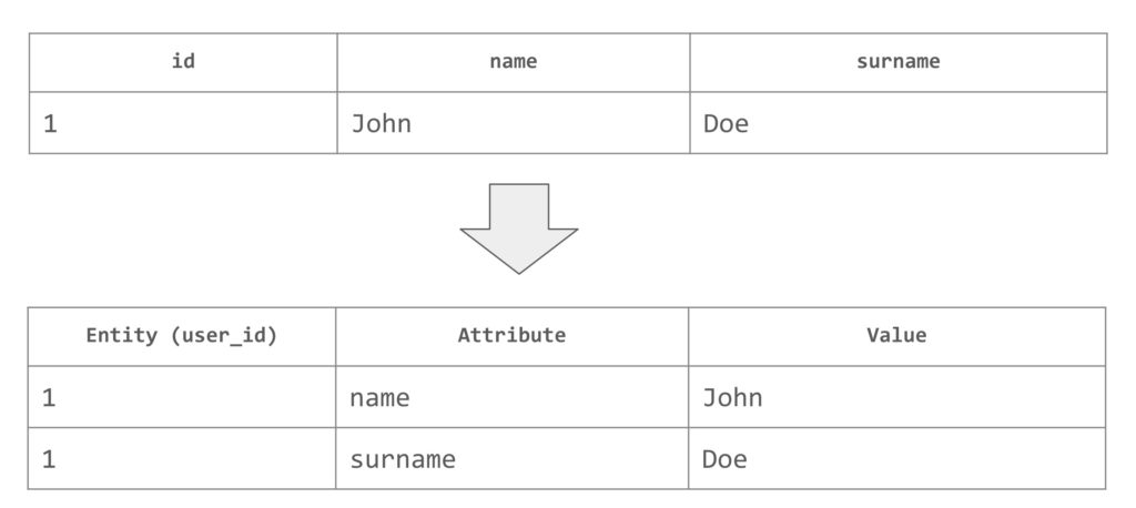
Fig. 1: EAV model and its transformation into regular table

We will demonstrate the use of CTEs in combination with the Entity-Attribute-Value (EAV) model. In this model, data is stored as three columns: an entity unique identifier, an attribute name, and an attribute value. This allows for a fully dynamic data model in relation to the database without the need for schema changes. An example of the EAV model can be seen in Fig 1. In connection with the EAV model, pivoting is often required. Pivoting enables us to transform EAV data into a regular table (Listing 15), and this is where CTEs come into play.

SELECT user_id,
   MAX(CASE WHEN meta_key='first_name' THEN meta_value END) as first,
   MAX(CASE WHEN meta_key='last_name' THEN meta_value END) as last
FROM `wp_usermeta`
GROUP BY user_id

+---------+--------+---------+
| user_id | first  | last    |
+---------+--------+---------+
|       1 | Emma   | Obrien  |
|       2 | Nial   | Casey   |
|       3 | Keeley | Brookes |
|       4 | Bert   | Mccoy   |
|       5 | Alyce  | Sheldon |
+---------+--------+---------+

We can use a pivoting query as the base for a CTE table. A CTE is built around the following pattern: “WITH name of cte table AS (query that will be used as base for cte) query that will be executed on cte table“. After filling the CTE table with result of pivot operation, we should execute a query that selects data from the CTE table (Listing 16).

WITH cte AS (
   SELECT user_id,
      MAX(CASE WHEN meta_key='first_name' THEN meta_value END) as first,
      MAX(CASE WHEN meta_key='last_name' THEN meta_value END) as last
   FROM `wp_usermeta`
   GROUP BY user_id
)
SELECT * FROM cte
WHERE first = "Emma" OR last = "Sheldon"
ORDER BY first

There is also a special recursive variant of CTEs in which the subquery refers to itself. This approach can be used to generate time series or traverse hierarchical or tree-structured data (Listing 17). In this case CTE is extended by the RECURSIVE modifier. A CTE query is also a bit different and is now made up of two parts or members: seed and recursive. Both are connected with the “UNION ALL” statement. The seed member represents the initial query, executed in the first iteration. The recursive member refers to the same CTE name (hence is recursive) and generates all remaining rows for the main query during execution.

WITH RECURSIVE cte AS (
   initial_query    -- "seed" member
   UNION ALL
   recursive_query  -- recursive member referring the same CTE
)
SELECT * FROM cte;  -- main query

A demonstration of this can be seen in Listing 18, where we generate a list of ascending dates starting with the date from the seed member (1.1.2013) and subsequently increase this value by one day in a recursive query until we reach the specified condition in the query. The last part of the query is a plain select from the CTE table.

WITH RECURSIVE cte (n) AS
(
  SELECT '2013-01-01'
  UNION ALL
  SELECT n + INTERVAL 1 DAY FROM cte WHERE n < '2013-01-10'
)
SELECT * FROM cte;

+------------+
| n          |
+------------+
| 2013-01-01 |
| 2013-01-02 |
| 2013-01-03 |
| 2013-01-04 |
|     …      |

One of the most powerful uses of a recursive query is retrieving a tree structure from a database. We will demonstrate this with a list of pages in Listing 19. Each page has a parent represented by its parent id. We start by selecting the parent element (“Home”), which does not have any other parent, for the seed member. In the recursive part, we select the record from the “page_cte” and join it with the “pages” table. We can then use the values from “page_cte” to create things such as breadcrumbs: “CONCAT(pc.path,’ -> ‘,pg.name)” or to show the item level: “rc.level + 1“.

CREATE TABLE pages(
   id         INT PRIMARY KEY AUTO_INCREMENT,
   name       VARCHAR(20),
   parent_id INT,
   FOREIGN KEY (parent_id) REFERENCES pages(id)
);

WITH RECURSIVE pages_cte(id, name, path, level) AS (
   SELECT id, name, CAST(name AS CHAR(100)), 1
   FROM pages
   WHERE parent_id IS NULL
   UNION ALL
   SELECT pg.id, pg.name, CONCAT(pc.path,' -> ',pg.name), pc.level+1
   FROM pages_cte pc JOIN pages pg ON pc.id=pg.parent_id)
SELECT * FROM pages_cte ORDER BY level;
+------+----------+---------------------------------------+-------+
| id   | name     | path                                  | level |
+------+----------+---------------------------------------+-------+
|  1   | Home     | Home                                  |     1 |
|  2   | Articles | Home -> Articles                      |     2 |
|  3   | Events	  | Home -> Events	                     |     2 |

Window functions

Windows functions [9] offer aggregate-like functionality on a defined range of rows in a query and were introduced in version 8.0.2. The main difference is that they return a value for every row in the query result, in contrast to regular SQL aggregations, which collapses the rows automatically. Windows functions are built around two key words: “OVER“, which is mandatory and indicates the usage of a window function, and “PARTITION BY“, which is used to divide the rows into groups (Listing 20).

SELECT
   <agregation>(field) OVER() AS field_name,
   <agregation>(field) OVER(PARTITION BY field) AS field_name
FROM <table name>

Window functions

The following example demonstrates the use of windows functions on the “transactions” table, which holds information about sales across countries and products. One can query the table for statistics using regular aggregations (Listing 21) or a window function (Listing 22).

CREATE TABLE transactions(
   id      INT PRIMARY KEY AUTO_INCREMENT,
   year    INT,
   country VARCHAR(20),
   product VARCHAR(32),
   profit  INT
);

SELECT SUM(profit) AS total_profit FROM transactions;
+--------------+
| total_profit |
+--------------+
|         7535 |
+--------------+
SELECT country, SUM(profit) AS country_profit 
FROM transactions GROUP BY country ORDER BY country;
+---------+----------------+
| country | country_profit |
+---------+----------------+
| Finland |           1610 |
| India   |           1350 |
| USA     |           4575 |
+---------+----------------+

Both solutions return the same values representing the total profit and profit aggregated by country, but the window function does not collapse the result and returns every row.

SELECT
   year, country, product, profit,
   SUM(profit) OVER() AS total_profit,
   SUM(profit) OVER(PARTITION BY country) AS country_profit
FROM transactions
ORDER BY country, year, product, profit;

+------+---------+------------+--------+--------------+----------------+
| year | country | product    | profit | total_profit | country_profit |
+------+---------+------------+--------+--------------+----------------+
| 2000 | Finland | Computer   |   1500 |         7535 |           1610 |
| 2000 | Finland | Phone      |    100 |         7535 |           1610 |
| 2001 | Finland | Phone      |     10 |         7535 |           1610 |
| 2000 | India   | Calculator |     75 |         7535 |           1350 |
| 2000 | India   | Calculator |     75 |         7535 |           1350 |

Usability may be questionable at first glance, but there are other window functions such as “RANK“. The “RANK” function can be used to assign rank to individual rows. Next interesting function is “FIRST_VALUE“, which represents the first value in the result set and can be used to calculate the difference between the value of the first row and other rows, as shown in example Listing 23.

SELECT
   year, country, product, profit,
   RANK() OVER(
      PARTITION BY `country`
      ORDER BY `profit` desc, id
   ) total_profit_rank,
   profit - FIRST_VALUE( profit ) OVER (
      PARTITION BY `country`
      ORDER BY `profit` desc, id
   ) profit_back_of_first
FROM transactions
ORDER BY country, total_profit_rank;
+------+---------+------------+--------+-------------------+----------------------+
| year | country | product    | profit | total_profit_rank | profit_back_of_first |
+------+---------+------------+--------+-------------------+----------------------+
| 2000 | Finland | Computer   |   1500 |                 1 |                    0 |
| 2000 | Finland | Phone      |    100 |                 2 |                -1400 |
| 2001 | Finland | Phone      |     10 |                 3 |                -1490 |

These are not the only functions available. For a complete list of functions, refer to documentation. [10]

IPC NEWSLETTER

All news about PHP and web development

Closing notes

The latest versions of MySQL are packed with surprises, and even patch versions can introduce intriguing features. It is important to always check which patch version is being used and to consult the documentation and release notes. But above all, don’t be afraid to harness the full power of new features in MySQL!